Grupo Experimental de Núcleos y Partículas

Welcome on the Home Page of the Run 107 and Run 119

These experimental runs consists of these experiments:

S 184: ¹³⁶Xe+p at 200, 300, 500, 1000 and 1400 A MeV
Energy dependence in the spallation of ¹³⁶Xe
(PhD thesis of Paolo Napolitani)

S 227: ¹³⁶Xe+Be at 1000 A MeV
Exploring the Production of Neutron-rich Isotopes by Cold-Fragmentation Reactions
(Jose Benlliure)

S 266: ¹³⁶Xe+Pb; ¹²⁴Xe+Pb at 1000 A MeV (February 2004)
Determination of the Freeze-out Temperature by the Isospin Thermometer (PhD thesis of Daniela Henzlova)
Longitudinal Momentum Distribution in Mid-peripheral Relativistic Heavy Ion Collisions (PhD thesis of Vladimir Henzl)

NOTE: this web is being actualized for the continuation of the S266 with ¹²⁴Xe beam !!! (see the "Latest News")

Latest News

Experimental Setup

Technical Info

Pictures

Estimated Xs

FRS Calibration

Settings

Brho estimations

Charge states

Participants

Shifts

Related links

Run 119

Latest News

February 5th, 2004, 15:54
Due to the high priority of HADES and the consequences of the SIS fire two weeks ago, our beam time has been shortened by one day, but stays almost as originally scheduled. According to the most recent information, the ¹²⁴Xe beam will be available for us between February 19th to 23th.

January 29th, 2004, 16:50
According to the latest info from the beam time coordinator, it is possible that the S266 experiment will be delayed by app. 1 week. The reason is the high priority of  HADES which may be put forward. Otherwise, the experiments during the "no-beam" period would be canceled and the rest scheduled as before.

January 29th, 2004, 16:43
This web page has been resurrected in order to provide information base for all participants of the new experimental run, continuation of the "S266 Isospin thermometer" experiment.

November 15th, 2002, 1:10
200 MeV is over, we launch the new energy 500 AMeV ¹³⁶Xe+p.

November 14th, 2002, 13:53
Enrique becomes father . The son is named Anton and was born with mass of m=3.5x10³ g

November 14th, 2002, 9:39
Beam is back , problems with the extraction solved. We can continue with the experiment.

November 13th, 2002, 18:50
The problems with the extraction cause an interruption of the experiment. The night shift of the C team has been canceled. The first possibility for the new (and better beam) is around 8:00-9:00 tomorrow morning.

November 13th, 2002, 16:20
We officially informed HKR and the beam coordinator that without the problems of the extraction being fixed, we cannot continue with the experiment.

November 13th, 2002, 15:50
The extraction of the beam from SIS became very bad and unsuitable for our experiment. Even for counting rate of 100 counts per second, dead time is more than 50%. It seems there are some severe problems with the extraction device which need to be repaired.

November 12th, 2002, 0:55
S227 is over. We switch to 200 AMeV and after few days continue with S184 spallation experiment.

November 11th, 2002, 2:00
We have put some pictures on the web.

November 10th, 2002, 15:22
S227 cold fragmentation experiment is launched.

November 10th, 2002, 15:21
The shared calibration is finished, S266 experiment is over.

November 10th, 2002, 11:55
The last measurement with Pb target is finished. The calibration shared by S227 and S266 starts.

November 8th, 2002, 2:40
First part of the S184 (¹³⁶Xe+p at 1 AGeV) experiment is finished. The S266 (¹³⁶Xe+Pb) is launched.

November 4th, 2002, 13:32
Change of the source to the enriched sample.

November 4th, 2002, 12:15
FRS Calibration page has been also filled on this web.

November 4th, 2002 0:52
First experimental setting with Hydrogen target. "The real thing starts :-)"

November 2nd, 2002, 22:26
We have the first beam !!!!

November 2nd, 2002, 16:45
The proposed values of high voltages for Multi-Wires (based on the experience of Run106) have been put on the web.

November 2nd, 2002, 15:10
Paolo's setting can be found on his page. This is still supposed to be a preliminary version only.

November 1st, 2002, 20:32
First version of "Run107 participants phonebook" has been released.

November 1st, 2002, 18:30
First beam expected sometime between Saturday evening (02/11/02) and Sunday morning (03/11/02).

November 1st, 2002, 18:00
S2 and S4 areas have been closed. The only possibility to access now is with the activated badge. Never enter alone !!!

November 1st, 2002, 16:14
First beam will be ^natXe. It can be changed to enriched ¹³⁶Xe the earliest on Monday (04/11/02)

November 1st, 2002, 16:10
Beam expected on Sunday morning (03/11/02) at around 6:00a.m.

November 1st, 2002, 16:08
This page of "Latest news" have been launched. All the events and news older than this page are not displayed.

return

Experimental Setup

return

Technical Info

FRS ion optics

• theory of ion optics

• ion optics details in Run107

Layers of matter

• List of layers of matter in the beam line and their estimated (not calibrated !!!) thickness

Detectors and electronic

• experimental layout

• beam profile monitors

• MUSIC chambers

• scintillators

• multiwire proportional chambers

• SEETRAM and its calibration

• general hints and useful remarks

Data acquisition

• MBS: (Multi Branch System)

• DAQ handling

• on-line analyses (Satan, Paw)

• parameter list

FRS handling

• before starting

• setting the FRS

• saving a setting

• routine duties

• procedures to open/close FRS-caves

• various useful "How to's"

Theory of Ion Optics:

• Nice and comprehensive of the basic ion optics supported by mathematical equations together with their derivations written by This email address is being protected from spambots. You need JavaScript enabled to view it..

• If you don't trust to Paolo or you find all his precise equation to be too complicated and rather too confusing, then try the lessons of Karl-Heinz Schmidt given to This email address is being protected from spambots. You need JavaScript enabled to view it..

Ion optic details for Run107:

• some more details about our Run107 to be added later ...

return

Layers of matter:

This Paolo's list of layers is also available for download as a "*.txt" format file.

Detectors

Experimental layout: to get an overview of the detector and electronic layout, you may take a look at the complete layout. If you want to take a look at one specific focal plane and the devices installed there, you choose one of the following S0 (target area), S1, S2, S3, S4.

Beam profile monitors: At the very beginning and during the calibration measurements you should check the profile of the beam. For this purpose  the beam monitors (referred to as the current grids) have been developed.

Music chambers (new and Munich):

• the general description of the MUSIC can be found at dedicated page of K.H.Schmidt.
• some more hints and remarks were also provided by K.H.Schmidt.

3-SCINTILLATORS

Multiwire proportional counters: proposed values of HV for MW; based on the Run106. 5-Seetram + IC a SCI calibracni.

General hints and useful remarks: these are the notes of Alexandra Kelic about all the detectors and electronic and the way have they are used or at least should be used.

Current Grids

Beam-Profile Monitors with Gas Amplification and Current Readout for the Projectile-Fragment Separator

M.Wber, E.Roeckl, K. Rykaszewski, I Schall

In order to measure spatial distributions of primary and secondary beams at the Projectile-Fragment Separator (FRS) [1], profile monitors with gas amplification and current readout have bee developed. These monitors are called "current grids" in order to distinguish them from FRS components based on single-event readout such as multi-wire proportional chamber.

Each current grid can be moved into and out of the nominal beam position by means of a compressed-air activated feedthrough. The mechanical layout of the wire planes, the electrodes and the mounting inside the gas chamber is based on experience gained at GANIL [2], [3]. For measuring the horizontal (x) and vertical (y) intensity distribution of beam, two planes of parallel wires (77 wires/plane, 1 mm distance) are used, being mounted between metal-foil cathodes in a gas chamber. There are five such small-area current grids, namely at each of the two target positions, at the intermediate and the final focal points, and in the transfer line to the ESR; furthermoere, two large-area current grids are positioned downstream of the first and third dipole, which have 95 wires (2 mm distance) in one plane for determining the x distribution only (see fig.1). In fig.2a and fig.2b and in table 1, the most important information on the mechanical layout of the current grids is compiled.

Table 1: Mechanical parameters of the current grids

	small-area current grids	large area current grids
wires: planes wires/plane distance thickness material	X and Y 77 1mm 20µm gilded tungsten	X 95 2mm 20µm |gilded tungsten
windows: number thickness size material	2 50µm 115mm stainless steel	2 100µm 1994 x 194mm2 stainless steel
intermediate cathodes: number thickness material	3 10µm stainless steel	2 10µm stainless steel

Fig. 1: Positions of the current grids at FRS

The x and Y wire planes of each small-area current grid are divided into a central region with single-wire readout, and two side regions, where two wires are combined, so that the 77 wires of one plane are readout into 47 channels. For the large-area current grid, single wires are readout into 95 channels.

By means of four FET multiplexers, up to eight current grids can be connected to two current-measurement units and the related control unit (see fig.3a). The current-measurement unit (see fig.3b) consists of 48 charge sensitive amplifiers. One amplifier includes in principle two electronic steps, namely a current-to-voltage converter and an integrator. After the integration time t_i the integrator provides a voltage level U_a1^, which is proportional to the time average of the incoming current, U_a1 ~ 1/t_i Int(t₀,t₀+t_i)[I_e1(t)dt] and stores this level, until the analog multiplexer has read out all of the 48 amplifiers (t_store=5ms). The control unit is connected via the SE interface to the VAX computer and allows to select 2 x 48 channels for simultaneous visualization, to vary the gain between 2nA/V and 10µA/V, and to select integration times of 0.5ms or 5ms using software of the SD control system [4], [5].

Fig.2: Sketch of the (a) small-area current grid and (b) large-area current grid

Following iinitial measurements [6], with ²⁰Ne(150 MeV/u), the current grids have meanwhile been further tested with beams of ⁴⁰Ar(164, 200, 720 MeV/u), ⁵⁴Fe(139 MeV/u), ¹⁹⁷Au(620 MeV/u), and ¹³⁶Xe(760 MeV/u). Fig.5 shows as an example the intensity profiles of a 760 MeV/u ¹³⁶Xe beam on both types of grids using the software of the SD control system. Typical parameters of the current grids during these measurements were:

Table 2: Typical parameters of the current grids.

gas:	500-800mbar, P10 (90%Ar, 10%CH4)
voltage on the cathodes:	-100 to -400 V
integration time:	5ms
beam intensities:	8 x 103 - 108 ions/bunch
electronic gain:	2-100nA/V

In order to study the gas amplification and to determine the minimum number of detectable ions, systematical parameter investigation as a function of gas composition, gas pressure, and high voltage are planned for various ions and intensities.

Fig.3: Principles of the read-out electronics for the current grids (a) and principles of the current-measurement unit (b).

Fig. 4: Intensity profiles of a 760 MeV/u ¹³⁶Xe beam from SIS. Shown are the vertical distribution measured with the current grids TS3DG2H (a), and the horizontal (b) and vertical (c) distributions measured with the current grid TS2DG2. The bunch width of the slowly extracted beam was approximately 600 ms, and the electronic integration time was 5 ms.

References

[1] H. Geissel et al., Projectile-Fragment Separator, A Proposal for the SIS-ESR Experimental Program (1987), unpublished
[2] D. Bazin and Y. Bouveret, Etude et mise au point d'une chambre multifits a ionisation pour la detection de faisceaux secondaires au GANIL, GANIL Report 84.03 (1984), unpublished
[3] R. Anne and Y.Georget, Chambres a a circulation de gaz, etalonnage avec le faisceau GANIL, GANIL Report RA.YG.627.85 (1985) unpublished
[4] M. Fradj, Beschreibung Profilgitter-Messsystem, Internal GSI-Report (1989), unpublished
[5] V. Schaa. Kurzbeschreibung SD-Anwahlprogramm, Internal GSI-Report (1990), unpublished
[6] R. Anne et al., Developement of Beam-Profile Monitors with Gas Amplification and Current Readout for the SIS Projectile-Fragment Separator, GSI Scientific Report (1990) p.257

return

Some hints on the use of the MUSICs

(Karl-Heinz Schmidt, 25. 9. 2002)

High-volt age supply

The high voltage of the cathode is supplied by a low-pass filter in order to reduce the wiggles originating from the power supply.

The anode is subdivided in 4 central anodes which are connected to one pre-amplifier each and 2 dummy anodes, closest to the entrance and the exit of the detectors. The charge collected on the dummy anodes is not collected, because the electric field in the vicinity of the field cage is not sufficiently homogeneous.

The dummy anodes receive their high voltage through a low-pass filter, which again serves to reduce the wiggles on the voltage from the power supply.

The inner anodes receive their high voltage through the pre-amplifiers. The pre-amplifiers are equipped with a low-pass filter, through which the high-voltage is connected to the input connector of the pre-amplifier.

The Frisch grid is connected to ground.

In figure 1, the high-voltage connections to the MUSIC are marked in red colour.

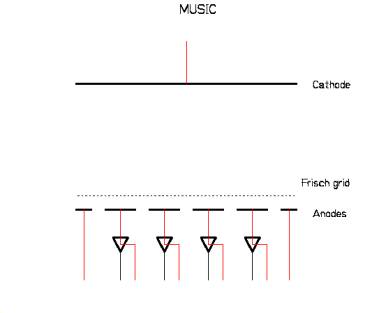
Figure 1: Electric connections of the MUSIC detectors. The high-voltage connections are marked in red, the signal connections in black.

Pre-amplifiers

The pre-amplifiers used to read out the energy-loss signals of the MUSICs consist of a charge-integrating operation amplifier, followed by a driver stage. The values of some key elements of the pre-amplifiers are important for their response to the input signals, for the noise, for the pile-up behavior and other important characteristics. They should carefully be optimized for any specific application.

A simplified layout of the pre-amplifiers is shown in figure 2.

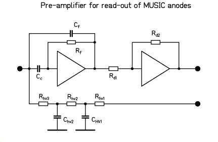
Figure 2: Schematic drawing of the most important components of the pre-amplifiers.

The following requirements have to be met:
C_f = 1 pF
C_f ´ R_f = 50 ms, consequently R_f = 50 MOhm.
R_hv3 > R_f
R_d1 = R_d2 (No pulse shaping and no amplification in driver section.)
R_hv1 + R_hv2 + R_hv3 should be small enough that the current from the ionization by the ions induces a drop of voltage less than a few Volts.
All capacities shown in figure 2 must be suited for the high voltage applied to the anodes (with a reasonable margin of security).

Quantitative estimate of the feedback capacity

As an example, we consider ¹³⁶Xe ions with an energy of 150 A MeV. The energy loss in Argon, 10 cm length, at atmospheric pressure is 176 MeV. This gives a charge of

q =176´10⁶ eV / 30 eV ´ 1.6´10^-19 As =9.4´10^-13 As.

For a feedback capacity of 1 pF this would lead to an output voltage of

U = 9.4´10^-13 As / 10^-12 F = 0.94 V.

Quantitative estimate of the current supply for the anodes

With a frequency of 10⁴ s^-1 this leads to an average current of

i = 9.4´10^-13 As ´ 10⁴ s^-1 = 9.4 nA.

To limit the variation of the voltage at the anodes to less than 10 V, the sum of the resistors

R_hv1 + R_hv2 + R_hv3 should be smaller than 10⁹ Ohm.

MW high voltages

Values of high voltages for MWs as they were used in Run106 by Klaus Suemerer et al.

MW11	2200 V
MW21	2100 V
MW22	2100 V
MW31	2200 V
MW41	2000 V
MW42	2300 V

Alexandra`s notes

return

Detectors and Electronics - hints

(AK 8.10.2002)

Detectors

1.      SEETRAM: current digitiser situated in the target area; upper limit 10⁴ counts/sec; sensitivity and offset of the digitiser are controlled from the Messenhutte (MH); the output of digitiser is sent to scaler (24 bits) situated in MH.

2.      SCINTILLATOR: used only for the calibration of SEETRAM; the output of PM is sent to discriminator (in MH) and than to 24-bit scaler; one should check the threshold of discriminator.

3.      IONIZATION CHAMBER: the output from PA is sent to amplifier (in MH); the amplitude signal from amplifier is digitised by ADC (2 or 4 KHz); the signal from amplifier is also sent to discriminator and than to scaler (24 bits); input from PA can be also sent to current digitiser (because of the higher signal compared to SEETRAM the sensitivity of this digitiser should be lower), and than to scaler in MH; sensitivity and offset of the digitiser can be controlled from MH.

4.      MULTIWIRES: MW11 at S1, MW21 and MW22 at S2, MW31 at S3 and MW41 and MW42 at S4; MW’s at S1, S2 and S3 are there only for calibration and beam positioning; except MW42, all others are in vacuum; anode lines are at 45^o, no delay lines in between; vertical and horizontal lines (x and y) are connected through delay lines; all signals from PA are sent to TDC (in MH), with anode signal as start signal and other four (x_l, x_r, y_u, y_d) as stop signals; exception, at S2 only the anode signal from one MW is used as start and all eight signals as stop.

5.      SCINTILLATORS: time and position information; at S2 only x information; at S4 possibility to use different scintillators giving the information on only x-position or on x- and y-position; TOF is obtained form the difference of signals from SCI21 and SCI41.

In principle, one can obtain the information on the energy loss from scintillator:

6. Music’s: two MUSIC at S4, both horizontal; each of 4 anodes gives two kinds of information: energy loss and drift-time; signal from PA is sent to main (t = 0.5 ms) and fast amplifier (with shorter time constant); signal from main amplifier is digitised and gives the energy-loss information, while the signal from fast amplifier is sent to CFD and than to TDC giving the drift-time information; this CFD has longer time delay than one of scintillator because of longer signal; all eight time signals (two MUSIC with four anodes) are stop signals for TDC, start signal is given by master trigger:

Problem of delta-electrons: small-impact collisions lead to high energy transfer, while large-impact collisions are leading to small energy transfer; in first glance, small-impact collisions are more preferable, but in reality they are destroying the energy resolution; this is the pure consequence of the statistical nature of the collisions: statistically, larger number of small-energy transfer signals will result in better resolution than a few high-energy transfer signals; high-energy transfer collisions result in more energetic electrons which travel longer distances and create secondary electrons; thus, the created electron-cloud has much larger dimensions than one created by slower electrons; as the consequence, high-energy events create tails in the PA output signal; these tails must be filtered and one should carefully choose MA time-constant in order to obtain good energy resolution:

stability of MUSIC: pressure and temperature can varie, and this can cause  wrong Z identificaton: change of 20 mbarrs in pressure results in DZ = 1; thus, one should make (in future) first order corrections for T and p on-line; in principle, not more than 1 KHz[1] counting rate with heavy ions can be supported by MUSIC (seen with fast PA); for higher rates charge resolution is destroyed:

Triggers and dead-time - master trigger is given by a passage of an in-coming particle; this trigger can be given by two different detectors: in the case of the data measurements by the SCI41_left, and in the case of the calibration measurements by SCI21; before the master trigger, all ADC’s are closed and only after the arrival of the particle the gate is opened during which ADC’s accept signals; in the case of TDC’s there is no gate, but the start of a TDC is put in coincidence with the master trigger.

After date being accepted, they are digitized; the conversion time is of the order  50-100 ms for old ADC’s and about 7 ms for Phillips ADC; the fastest conversed data are than read first and the slowest one last; time needed to digitize certain data should be taken into the account when writing the read-out program for front-end computer; after reading data are sent to PC and than to the GSI net and tapes.

While processing data (conversion, read-out) no other particle can be accepted; this is why a veto signal is imposed to master-trigger.

After reading all data and before accepted new particle, all ADC’s and TDC’s must be reset to zero; note: they are reset to zero only after the last channel is read. If there is no input in the last channel of ADC or TDC it will not be reset!

Dead-time of DAQ is determined by the number of free-triggers and number of accepted-triggers.

[1] C. Scheidenberger said that in the 900 A MeV ²³⁸U run in July 2002, at 10 KHz counting rate still the charge- resolution was good.

return

Data acquisition

MBS: (Multi Branch System)

• This is the standard Data Acquisition System at GSI. If you have some experience and would like to learn some fine details, then the best would be to visit the original MBS home page.

• If you are a beginner, who knows almost nothing about it and would like to start with it, or if you are someone who is forced to use it but don't know how (and official documents are too confusing and boring), well then try this friendly page.
  

DAQ handling:

• The best way how to learn handling of Daq is to read the Run107 Cookbook, which is based on the previous experiences gained during the Run98.

Online analyses (Satan, Paw):

• Before you can start any online analyses, you have to get connected to the Remote-Event-Server.

• Even if you get successfully connected, it brings no good unless you have an adapted online program for Satan (or Paw). The latest version of the online program used for the Run107 has been also provided by some useful comments and explanations for those who really want to learn and understand what they are doing (and not what is done for them by a program itself).

• If you already work with the Satan online, some description of all defined analyzers may come to a need.

• If you are the Paw user, then the best contact person is probably This email address is being protected from spambots. You need JavaScript enabled to view it., but some hints you can also find on our Paw online page.

Parameter list:

• the order of the read data (so called "parameter list"), e.g. the order of the 16bits words from the detectors and scalers in the way how they are read, recorded and send to clients.

return

FRS handling:

Before starting: loading ion-optical files, starting different programs.

On AXP316 (Program SD):

• click on SONDEROPTIONEN

• click on THEORIEWERTE SETZEN (Magnete)

• click on Prg Start

  the list of theoretical values for magnets and quadrupoles appears

• choose your theoretical data file by clicking

• click on Anzeigen to check that the file corresponds to what you expect (the magnets values appear on the window created by the program) when you are sure this is the file you wanted.

• click on Setzen to set the currents on the magnets.

• then go to program MGSKAL to scale all magnets (from SIS to S4 ).

Setting  the FRS

General remarks

All the programs used to drive magnets are available at the VT100 screens at the FRS cosole.
The simplest way to drive a magnet uses the program STRAHLFUEHRUNG UND DIAGNOSE running at the console workstation screen. Clicking the left key of the mouse at a specific section of the FRS given in the top line (TE1... to HFS1...) brings the magnets of this section on the potiboard. The potiboard allows to read "Ist" values and "Soll" values (the current and want-to-have values), and allows to modify the "Soll" values. However, this procedure is useful only for small adjustments of single magnets, e.g. for steering, and to check the actual setting.
In general, the setting of the magnets is modified using special programs, described below.

Procedures to change the setting (i.e. to scale the magnets)

!!! NOTE !!!: There are only 2 keyboards for the 5 terminals. To get the connection keyboard-terminal, use the button on the right.

1) Advise the person responsible for recording on tape to close the file

2) Stop the beam (SD.EXE + red button)
2.1) put in beam plug
2.2) close S1 horizontal slits

3) Load the reference setting (SRMAG - Save und restore magnetwerte)
3.1) go to MENU
3.2) go to DATENSATZE
3.3) go to SUCHKRITERIEN (if it is the 1st loading) and choose the reference setting (i.e. the reference file)
3.4) press the "Do" key in the keyboard
3.5) go to DATENSATZELADEN to load it
3.6) go to SAVE SETZEN
3.7) answer "J" to the question "Magnetwerte setzen?"
3.8) press "Do" key in the keyboard (!!! if the selected "Ersten Magnet" and "Letzten Magnet" are not OK change them and press "Do")
3.9) answer "K" to the question
3.10) answer "N" to the question "Fehlerprotokoll drucken?"

4) Choose the FRS section to be scaled MGSKAL (Magnetscaleriung) - !!! you have to change the terminal !!!
4.1) go to MENU
4.2) go to ENDE
4.3) go to AUSWAHL DER GRUPPE to choose the section
4.4) choose the section (TA_S2 or S2_S4)

5) Scale the section MGSKAL
5.1) go to SKALIEREN UND SETZEN
5.2) go to SKALIEREN MIT FACTOR
5.3) enter the scalling factor (evalueted with the Lieschen calculation)
5.4) answer "J" to the question "Magnetwerte setzen?"(return)
5.5) wait until the magnetic fields are stabilized

6) go to number 4 and redo the procedure until all is scaled (both sections TA_S2 and S2_S4 ???)

7) print the magnet status (SD.EXE)
7.1) click with the mouse on MAGSTAT

8) Start the beam (SD.EXE + green button)
8.1) move out beam plug
8.2) open S1 horizontal slits

9) Advise the person responsible for recording on tape to open a new file

Saving a setting

If you want to save some setting, use program SRMAG (at terminal 4)

1) go to ABSPEICHERN
2) go to the line which describes your experiment
3) be sure that there are no errors (Feller) in the reading
4) write a comment regarding the beam and beam-line status
5) write the initials of the people in shift (Schichtmannschaft)
6) write a keyword (Schüsselwort); this will be the name of this setting
7) press the "Do" key in the keyboard to save all
8) go to MENU

Routine duties: what to do during your shift.

Magnets

1) check that the calculations of the scaling factors are prepared (printed and stored in the folder)
2) if not, do (in advance) these calculations
3) be sure that the file has been closed
4) be sure that the beam has been stopped
5) scale the magnets (see the detailed procedure)
6) advise the person responsible to open/close files that magnets are changed and that a new file can be open

Main screen

1) control that the layers in the beam line are exactly those ones that are supposed to be there
2) be careful to the beam intensity when BRho is close to the primary beam and when you sweep the beam to the position of the slits (when they are needed)

Logbook

- write EVERYTHING what is happening in the logbook, please, detailed and in the way that it can be read by all the others

File sheets (open/close files)

1) open/close file when the person responsible for the scaling magnets advises you
2) write ALL (!!) the information in the file sheet
3) print the status of the magnets (or ask the person responsible for the scaling of the magnets to print it) and store it in the folder

On-line analysis with SATAN or PAW

1) check that all the used detectors are responding
2) check that the spectra look as they should be

Supervision

1) supervise everything
2) give instructions in case of not-routinely procedure
3) go to the meeting of the people of the accelerator group, at 12:45 in the "freezer"

Procedures to open/close FRS-claves

• how to open the caves when beam is on.

• how to enter the FRS vaults

• how to close the caves after a beam-off period

(KC2$ROOT:[PROFI.MANUALS]safety.tex)

1. How to open the caves when beam is on

Switch off dipoles TS3MU1  and TS3MU2 (SD-screen: click "AUS", then click both devices at the pictogram line. the green dipole symbols must turn red).

Close slits TS3DS2HL and TS3DS2HR by clicking the dot corresponding to TS3DS2H at the SD screen (use middle key of mouse to check if you selected the right device). Drive motors separately (!) by clicking the "I" field ("innen") with the left mouse key.

Close beam plug TS3SV3 by clicking the corresponding green dot (device TS3SV3_P) on the SD screen in row "ANTRIEBE". The dot must turn red.

Call control room (Tel. 221) to turn off virtual accelerator #8 and to direct it to another vault (e.g. the main beam stop in vault HHD). Ask to provide controlled access to cave via the automatic sliding doors.

NOTE: Do not touch slits and beam plug once the interlock system is activated since this causes an emergency situation that can be cleared only by health physics!

2. How to enter the FRS vaults

You must have a badge with a bar code that is registered with GSI health physics. Once the access to the cave is permitted (yellow light "Controlled Access" on) you open the sliding door by pressing the button "door open". Stand on the yellow area on the floor. Enter date of you birthday at the eight keyboard ("ddmmyy", "enter"). Remove a dose meter from the top left shelve and put it into the lower left receptacle (readout station) if the green light "READY" is on. Move your badge with the bar code up below the bar code reader at the right receptacle. Wait till the green light "OK" is on. Now you can remove the black dose meter and take it with you into the vault.

When returning from the vault, proceed the same way as above. After removing the black dose meter from the readout station put it back to the storage shelve above. The system will store any dose you gave received when in the vault.

3.  How to close the caves after a beam-off period

When all persons have left the vault, call the SIS operator (Tel. 211) and tell them to reactivate the virtual accelerator #8 and direst it to the FRS (target "HFS").

Switch on dipole TS3MU1 on the pictogram line (click "EIN", click red dipole symbol).

Remove beam plug TS3SV3 by clicking the corresponding red symbol on the line "ANTRIEBE" on the SD-screen.

Open the slits TS3DS2HL and TS3DS2HR as above by clicking the "A" ("aussen") fields separately.

Various useful "How to`s"

• how to change the Seetram sensitivity

• how to print magnet and detector status in Run107

How to change the SEETRAM's sensitivity

1) load the programm NODAL
2) run INTMON
3) choose the detector type (3)
4) choose the SEETRAM name (3)
5) choose the virtual accelerator (8)
6) choose 20 to check
7) choose 22 to change the SEETRAM sensitivity

Note: SEETRAM factor = 304.3 at sensitivity 10^-10

How to print magnet and detector status in Run107

set host AXP310
login: FRS
password: FSOPER
[FRS]$ cd [frs.ufc.run107]

! the following lines should be repeated
! for each printed files

[..RUN107]$ NODAL
> RUN FRS_status_read
Please enter Filename [for example F_02] : Fxxx
.
.
.
> quit
[..RUN107$ @printstat Fxxx

return

Estimated Xs

S 184 estimated cross sections:

• Paolo's experiment ¹³⁶Xe + p at 200, 300, 500, 1000 and 1400 A MeV

S 227 extimated cross sections:

• Jose's experiment ¹³⁶Xe + Be at 1000 A MeV

S 266 estimated cross sections:

• Daniela's and Vlad's experiment ^124,136Xe + Pb at 1000 A MeV

Below are displayed the estimated cross sections of fragments with Z=10, 20, 30, 40 and 50. The error bars are based on the expected statistics (1.10^{8 136}Xe ions per second beam intensity assumed). The cross section estimations were made with the use of LIESCHEN.

return

FRS Calibration

Calibration operations prior to measurements

0) Preliminar checks

• Check the beam position and angle at S0 using the current grids.

• Check that all slits are out of the beam line.

1) Center primary beam at S2 and S4

Low beam intensity. No material other than the SEETRAM is inserted at S0 at this step, no material at S2

• Insert MW21 and MW22 in the line, center beam at S2. Go on tape.

• Remove MW21 and MW22, center beam at S4 using MW41.  Go on tape.

• Knowing the energy of the ions and the magnetic fields value, determine the effective radii of the dipoles.

2) Center primary beam at S2

Target relevant for the upcoming mesurements is inserted in the beam line (see table below ).

• Insert MW21 and MW22 in the line, insert the dummy target (or the main target if H target is not to be used). Center beam at S2. Go on tape.

• Estimate the thickness of the target inserted at S0.

• If the experiment main target is the H target, repeat the 2 previous steps replacing the dummy target with it.

• If a stripper foil must be used at S0, insert it in the beam now and repeat the 2 first steps.

3) Center primary beam at S2 and S4

Material at S0 is now in place and should be moved anymore.

• Insert the plastic scintillator at S2, center the beam at S4 using MW41. Go on tape.

• Estimate the thickness of the scintillator. Keep trace of the TOF spectra and of the MUSIC spectra for the TOF calibration and the MUSIC calibration (TOF dependency).

• If additional material is needed at S2 (stripper foil, degrader... - see table below ) repeat the 2 previous steps.

• Once all material is in the beam line, save magnetic fields values as the “reference setting”.

4) Measurement of nuclear reactions at S2

Keep the same setting as at the end of the previous step.

• Set trigger at S2. Go on tape.

5) Charge states measurements

• Insert MW11 in the beam and set trigger on it (in low energy settings, increase magnetic rigidity in order to see simultaneously as many charge states as possible). Go on tape.

• Remove MW11 from the beam line, repeat the previous step with MW31.

• Remove MW31 from the beam line, set trigger back at S4.

6) TOF calibration and MUSIC dependency on TOF

Several settings have already been measured with the successive introductions of matter at S2.

• Repeat step 3 using one or more degrader thicknesses. Go on tape.

• Put back standard layers of matter, reload reference setting.

7) Measurement of dispersions

To ensure a fine measurement of dispersions, a scanning consisting of 5 steps of 0.3% in the magnetic fields values is to be performed during the initial calibration phase. During subsequent calibrations, a 1% step should be sufficient.

• Introduce MW21 and MW22 in the beam line. Gradually change magnetic fields in the first part of the FRS. Go on tape for each increase of the fields. Remove MW21 and MW22 from the beam line.

• Gradually increase magnetic fields in the second part of the FRS. Go on tape for each increase of the fields.

• Gradually restore the fields in the first part of the FRS to the reference value. Go on tape for each decrease of the fields.

• Restore the reference setting.

8) Calibration of the position dependency from the MUSIC

• Explore different positions at S4 by manually changing the value of the last dipole just before S4. Go on tape during all this procedure.

9) SEETRAM calibration

• Insert the S0 plastic and/or the Ionization Chamber in the beam line. If the plastic is chosen, the beam should also be centered at S2 and data from S2 recorded,  in order to get an estimation of the total cross section at S0.

• Ask for progressive increase of the beam intensity.  Go on tape during all the increase of intensity.

• Above 100kHz insert the beam stop at S1 in order to protect the plastic at S2.

• Reload reference setting.

10) Calibration of the S2 and S4 scintillators

Beam intensity is now normal.

• Set trigger at S2 again. Insert MW21 and MW22 in the beam line. Set the magnets to cover a standard fragment setting, preferentially far from the projectile. Go on tape.

• Set trigger back at S4, remove MW21 and MW22 from the beam line.  Go on tape.

Repeat step 2, 3 and 5. Repeating also step 9 is a good thing in order to check SEETRAM stability.

Calibrations after a change of the beam energy

• All operations are to be done again, with the exception of step 8.

• Step 6 is not necessary if electronics is not changed and if the new TOF range has been covered in a previous calibration measurement.

• Step 7 can be done in a shorter way: instead of the cautious scanning per steps of 0.3%, a single step of 1% should be enough in the case of Xe beam.

• Repeat step 10 only if scintillator has been changed.

Layers of matter at S0 and S2 for the various measurements (expected values).

Measurement	Layers of matter at S0	Magnetic rigidity of beam in first section	Layers of matter at S2	Magnetic rigidity of beam in second section
Xe + p @ 1 GeV - heavy fragments	H target (or dummy target)	14.1182 (14.1957)	Scintillator 5mm	13.9695 (14.0475)
Xe + p @ 1 GeV - light fragments	H target (or dummy target)	14.1182 (14.1957)	Scintillator 3mm(?)
Xe + Pb @ 1 GeV	Pb target (635mg/cm²)	14.0416	Scintillator 5mm Degrader (816.6mg/cm²)	13.5044
Xe + Be @ 1 GeV	Be "thin" target (1023mg/cm + 221mg/cm² Nb backup) Be "thick" target (2526mg/cm²+ 221mg/cm² Nb backup)	13.7391   13.1386	Scintillator 5mm Nb stripper foil (106mg/cm²)	13.4832   12.8749
Xe + p @ 500 MeV	H target (or dummy target)	8.9913 (9.1044)	Scintillator 3mm Ti stripper foil (45mg/cm²)	8.7506 (8.8669)
Xe + p @ 200 MeV	H target (or dummy target)	5.1018 (5.3416)	Scintillator 1mm Al stripper foil (54 mg/cm²)	4.8741 (5.1318)
Xe + p @ 1.4 GeV - heavy fragments	H target (or dummy target)	17.8708 (17.9387)	Scintillator 5mm	17.6792 (17.7476)
Xe + p @ 1.4 GeV - light fragments	H target (or dummy target)	17.8708 (17.9387)	Scintillator 5mm Thin degrader

return

Settings

The general file sheet can be downloaded either as a standard Word "*.doc" file or as a standard "*.pdf" file.

S 184 settings: Paolo's experiment ¹³⁶Xe + p at 200, 300, 500, 1000 and 1400 A MeV.

S 227 settings: Jose's experiment ¹³⁶Xe + Be at 1000 A MeV

S 266 settings: Daniela's and Vlad's experiment ^124,136Xe + Pb at 1000 A MeV. List of files connected to S266 (calibrations + experimental settings).

return

Brho estimations

S184 brho estimations: Paolo's experiment ¹³⁶Xe + p at 200, 300, 500, 1000 and 1400 A MeV.

S227 brho estimations: Jose's experiment ¹³⁶Xe + Be at 1000 A MeV.

S 266 brho estimations: Daniela's and Vlad's experiment ^124,136Xe + Pb at 1000 A MeV.

SIS window + Seetram Ti: (5.0+3x4.5) mg.cm-2	natPb target Pb: 635.0 mg.cm-2	PPAC Al(eq): 110 mg.cm-2	Scintillator S2 (5 mm) Al(eq): 565.3 mg.cm-2	Degrader (rot.discs) Al: 816.6 mg.cm-2	Brho	Brho
Yes	No	No	No	No	14.2087	14.2087
Yes	No	No	Yes	No	14.2087	13.9922
Yes	No	Yes	Yes	No	14.2087	13.9498
Yes	No	Yes	No	No	14.2087	14.1668
Yes	No	No	No	Yes	14.2087	13.8955
Yes	No	Yes	Yes	Yes	14.2087	13.6327
Yes	No	No	Yes	Yes	14.2087	13.6757
Yes	Yes	No	No	No	14.0421	14.0421
Yes	Yes	No	Yes	No	14.0421	13.8240
Yes	Yes	No	Yes	Yes	14.0421	13.5050
Yes	Yes	Yes	Yes	No	14.0421	13.7813
Yes	Yes	Yes	Yes	Yes	14.0421	13.4617

return

Charge states

S184 charge state estimations: Paolo's experiment ¹³⁶Xe + p at 200, 300, 500, 1000 and 1400 A MeV.

S227 charge state estimations: Jose's experiment ¹³⁶Xe + Be at 1000 A MeV.

S266 charge state estimations: Daniela's and Vlad's experiment ^124,136Xe + Pb at 1000 A MeV.

SIS window + Seetram Ti: (5.0+3x4.5) mg.cm-2	natPb target Pb: 635.0 mg.cm-2	PPAC Al(eq): 110 mg.cm-2	Scintillator S2 (5 mm) Al(eq): 565.3 mg.cm-2	Degrader (rot.discs) Al: 816.6 mg.cm-2	0e-	1e-	2e-
Yes	No	No	No	No	0.99606	0.00394	0.00000
Yes	No	No	Yes	No	0.98855	0.01142	0.00003
Yes	No	Yes	Yes	No	0.98846	0.01150	0.00003
Yes	No	Yes	No	No	0.98939	0.01058	0.00003
Yes	No	No	No	Yes	0.98835	0.01161	0.00003
Yes	No	Yes	Yes	Yes	0.98780	0.01216	0.00004
Yes	No	No	Yes	Yes	0.98790	0.01207	0.00004
Yes	Yes	No	No	No	0.98924	0.01073	0.00003
Yes	Yes	No	Yes	No	0.98821	0.01176	0.00003
Yes	Yes	No	Yes	Yes	0.98752	0.01244	0.00004
Yes	Yes	Yes	Yes	No	0.98812	0.01185	0.00004
Yes	Yes	Yes	Yes	Yes	0.98743	0.01253	0.00004

return

Participants

return

Shifts

This is the version of the shift schedule made on October 29, 2002, Fanny, Jose and Andreas. Updated on October 31 (all shifts shifted by 8 hours).

Team					.
A	J.Benlliure	E. Casarejos	L. Audouin	M. V. Ricciardi	J.E. Ducret	M. Fernandez-Ordonez
B	A. Heinz	C. Volant	S. Leray	T. Enqvist	D. Henzlova	V. Henzl
C	F. Rejmund	A. Kelic	C. Stephan	A. Lafriakh	C. Schmitt	C. Villagrasa
D	A. Boudard	J. Pereira-Conca	O.Yordanov	L. Tassan-Got	P. Napolitani

	0:00 - 8:00	8:00 - 16:00	16:00 - 24:00
Saturday 2
Sunday 3	B	C	D
Monday 4	A	B	C
Tuesday 5	D	A	B
Wednesday 6	C	D	A
Thursday 7	B	C	D
Friday 8	A	B	C
Saturday 9	D	A	B
Sunday 10	C	D	A
Monday 11	B	C	D
Tuesday 12	A	B	C
Wednesday 13	D	A	B
Thursday 14	C	D	A
Friday 15	B	C	D
Saturday 16	A	B	C
Sunday 17	D	A	B
Monday 18	C

return

Related links

Run99 Home Page: The web page of Run99 created by Jose Benlliure. This page served as the inspiration for our Run107 web page. Still a lot of  interesting information can be found there.

Karl-Heinz Schmidt: The home page of Karl-Heinz Schmidt witch contains information relevant to experiments in the past same as to the future projects of the whole (=his) group. Great article and software tools library.

Valentina Ricciardi: The home page of Valentina. The most valuable is her PhD Theses (High-resolution measurements of light nuclides produced in 1×A GeV 238U-induced reactions in hydrogen and titanium) and many interesting notes and comments useful especially for the data analyses and work with AMADEUS and LIESCHEN.

Paolo Napolitani: Paolo's home page with a lot of information on his spallation studies and proposals for the Isospin thermometer project.

Daniela Henzlova: The web page dedicated to Daniela's PhD theses on the Isospin Thermometer.

Vladimir Henzl: Vlad's homepage dedicated to his PhD theses on the Longitudinal momentum distribution in mid-peripheral relativistic heavy ion collisions.

... maybe you think that some special link is missing here .... just let me know then !

return

Run 119

This run is the 2nd half of the Isospin Thermometer Experiment (S266)

Technical Info

Experimental details

Participants

Run 119 News

Technical info

Layers of matter: List of layers of matter in the beam line and their estimated (not calibrated !!!) thickness.

Data acquisition for Run 119

• MBS: (Multi Branch System).

• DAQ handling.

• on-line analyses (Satan, Paw).

• parameter list

FRS handling

• before starting

• setting the FRS

• saving a setting

• routine duties

• procedures to open/close FRS-caves

• various useful "How to's"

Detectors and electronics

• experimental layout

• beam profile monitors

• MUSIC chambers

• scintillators

• multiwire proportional chambers

• SEETRAM and its calibration

• general hints and useful remarks

 

Layers of matter in beam for two possible energies:

1000 A MeV (???) 500 A MeV
***************** S0 *************************************************************************************

SIS window (Z:22 A:47.9 D:5 [mg/cm**2])  

Seetram 0.03mm (Z:22 A:47.9 D:13.5 [mg/cm**2])

Pb target (Z:82 A:208 D:635 [mg/cm**2])
Pb target (Z:82 A:208 D:397 [mg/cm**2])

***************** S2 *************************************************************************************

MW21 (Z:13 A:26.98 D:165. [mg/cm**2])

Scintillator S2 3mm (Z:13 A:26.98 D:~400 [mg/cm**2])
Scintillator S2 5mm (Z:13 A:26.98 D:~600 [mg/cm**2])

MW22 (Z:13 A:26.98 D:165. [mg/cm**2]) (for calibrations only)

Rotating Wedges - degrader (Z:13 A:26.98 D:847 [mg/cm**2])

***************** S4 *************************************************************************************

MW41 (Z:13 A:26.98 D:165. [mg/cm**2]) 

FRS window (Z:22 A:47.9 D:90.2 [mg/cm**2])

Air (Z:7 A:14. D:~50. [mg/cm**2])

Music1 @ atm press (Z:18 A:40. D:100. [mg/cm**2])

Music2 @ atm press (Z:18 A:40. D:100. [mg/cm**2])

Scintillator S4 5mm (Z:13 A:26.98 D:~600 [mg/cm**2])

MW42 (Z:13 A:26.98 D:90. [mg/cm**2])

 

**********************************************************************************************************

DAQ handling: The best way how to learn handling of Daq is to read the Run119 Daq handling, which is based on the previous experiences gained during the Run98 and Run107.

Online analyses (Satan, Go4):

• Before you can start any online analyses, you have to get connected to the Remote-Event-Server.

• Even if you get successfully connected, it brings no good unless you have an adapted online program for Satan (or Go4). The Run107 version of the Satan online program has been also provided by some useful comments and explanations which hold for today as well. for those who really want to learn and understand what they are doing (and not what is done for them by a program itself).

• The Go4 online analyses program is being prepared by This email address is being protected from spambots. You need JavaScript enabled to view it..

FRS Handling

Before starting: loading ion-optical files, starting different programs.

Setting the FRS: loading a reference setting and scaling; the control of the magnets.

Saving a setting.

Routine duties: what to do during your shift.

Procedures to open/close the FRS-caves

• how to open the caves when beam is on.

• how to enter the FRS vaults.

• how to close the caves after a beam-off period.

Various useful "How to's"

• how to change the Seetram sensitivity.

• how to print magnet and detector status in Run107.

Experimental details

• The list of calibrations (and their brief description) prior or complementing the measurements.

• The settings of the Fragment Separator, estimated characteristics of the beam and length of the measurement for Run119.

• The file sheets are available for download as Word .doc file.

• Run 119 settings.
• Brhos in Run 119.
• Charge states.

Participants

Run 119 News

return